Iron — A Complete Market Guide (2026)

Data as of 10 October 2026. Iron ore market structure is shown for full-year 2025, the latest complete year, from the USGS Mineral Commodity Summaries 2026 (and its earlier editions for the history), worldsteel’s World Steel in Figures 2026, the Australian Government’s Resources and Energy Quarterly (September 2026), UN Comtrade and the producers’ 2025 annual reports; trade by country is for 2024, the latest year worldsteel prints country by country. Prices are full-year and multi-year averages of the World Bank’s iron ore series, not a single day’s quote, so this report stays useful over time; 2026 prices enter only as a clearly labelled aside. Every figure is traced to its source in the register at the end (Section 8.1). This report is for information only and was prepared with AI assistance — see the disclaimer at the end.

Iron ore is the raw material of steel, and so of every building, bridge, ship, car and machine on Earth. By tonnage it dwarfs every other mined metal: about 2.6 billion tonnes of usable ore were mined in 2025, and more than 1.7 billion tonnes crossed a border in 2024, most of it on ships bound for China. The market is at a turn: Chinese steel output peaked in 2020, the largest new high-grade mine in decades — Simandou in Guinea — shipped its first ore in December 2025, and decarbonisation is splitting demand between ordinary ore and premium grades. This report is the free, big-picture primer on how the iron ore market works: where the ore comes from, who buys it, how a negotiated benchmark became a daily index, and what drives the cycle. For the company-level data behind the story — every producer screened by production, reserves and cost — go to Metal Pilot’s iron ore mining stock screener.

TL;DR & Key Takeaways

• What it is: a rock rich in iron oxide — hematite or magnetite — and the only commercial source of new iron. Almost all of it is made into steel, so iron ore demand is steel demand one step upstream.
• Who supplies it: mines produced 2.6 Gt of usable ore in 2025; Australia mined 38% and Brazil 16%. Exports are even more concentrated: Australia and Brazil shipped 74% of world exports in 2024, and four companies — Vale, Rio Tinto, BHP and Fortescue — dominate both.
• Who uses it: China, which made 52% of the world’s 1,849 Mt of crude steel in 2025 and buys about 75% of seaborne ore. Its steel output peaked at 1,065 Mt in 2020; India is the large grower, and electric-arc furnaces fed by scrap make 30% of world steel.
• The balance: no agency publishes a surplus or deficit. The market is read through China’s imports — a record 1,238 Mt in 2024 — and Chinese port stocks, which reached 160 Mt at the end of 2025, about six weeks of imports.
• The price regime: pro-cyclical and China-geared. The benchmark averaged about $19 a tonne in 2000 in the contract era, $168 in 2011, $56 in 2015, $162 in 2021 and $100 in 2025 — against unit costs near $18–24 a tonne at the four largest producers.
• The swing factor: Chinese steel output against a new supply wave — Simandou’s ramp toward 120 Mt a year plus record output from the majors, arriving as Chinese demand declines.

Figure 1. Iron ore at a glance, 2025

Notes to Figure 1

1. Mine production — Table 10 · Filed · USGS MCS 2026 · World Mine Production and Reserves · “World total (rounded)" 2,600,000 (thousand metric tons, usable ore), 2025e · p.109.
2. 62% Fe price — Table 3 · Market · World Bank · “Iron ore, cfr spot”, annual · 2025. The latest full-year average; the trailing twelve months are in the aside under Figure 3.
3. Market size — Derived · 2,600 Mt (tile 1) × $100.2/t (tile 2) = $261 bn. An upper-bound proxy: not every tonne is benchmark grade or sold at the seaborne price. Exporters declared $148.4 bn of iron ore exports in 2024 (Table 16).
4. World crude steel — Table 9 · Filed · worldsteel WSIF 2026 · World crude steel production 1950 to 2025 · “World” 1 849 · p.7.
5. China’s share of seaborne imports — Table 12 · Filed · REQ September 2026 · Iron ore · “China imports 75% of global seaborne iron ore supply” · p.35.
6. Australia and Brazil’s share of exports — Table 16 · Derived · (901.6 + 389.2) ÷ 1,740.5 Mt, 2024 = 74.2%; worldsteel WSIF 2026, “Iron ore, 2024”, p.20.
7. Electric-arc share — Table 6 · Filed · worldsteel WSIF 2026 · Crude steel production by process, 2025 · “Total of above countries” electric 30.3% · p.10.
8. Reserve life — Table 11 · Derived · reserves 87,000 Mt of iron content ÷ 2025e mine production 1,600 Mt of iron content (USGS MCS 2026, p.109) = 54 years. On the crude-ore basis the reserves are 200 Gt, which cannot be divided by usable-ore output.

Figure data: Tables 3, 6, 9, 10, 11, 12 and 16 — USGS Mineral Commodity Summaries 2026: Iron Ore (page numbers are those of the full volume), worldsteel World Steel in Figures 2026, the Australian Government’s Resources and Energy Quarterly, September 2026 and the World Bank Pink Sheet; each tile’s citation is in the notes above.

Why it matters now: iron ore is entering its first structural transition since China industrialised. Supply is growing — Simandou plus record volumes from the majors — just as Chinese steel, half the market, declines, while low-carbon steelmaking raises the value of high-grade ore. For an investor, the world’s most profitable large-scale mining business is heading into a cycle where cost position and ore quality, not volume growth, decide the winners (Section 4).

How to read this guide: new to iron ore? Read straight through from Section 1. Here for the investment case? Jump to Section 4 — how to own it, how to screen the producers, and which regimes favour it. Every technical term is defined in the Vocabulary (Section 7).

1. Iron & the market basics

1.1 What iron ore is — physical basics & quality

Iron (chemical symbol Fe) is one of the commonest elements in the Earth’s crust, and iron ore is the only commercial source of new iron. Two minerals dominate. Hematite (Fe₂O₃) forms the rich deposits of Australia’s Pilbara and Brazil’s Carajás; much of it is direct-shipping ore (DSO) — ore that needs only crushing and screening before sale. Magnetite (Fe₃O₄) is usually lower-grade in the ground but magnetic, so it can be separated into very high-grade concentrate — the basis of Sweden’s Kiruna, the US taconite mines, Canada’s Labrador Trough and Fortescue’s Iron Bridge. Iron ore was never scarce geologically: world reserves are 200 billion tonnes of crude ore holding 87 billion tonnes of iron, against 1.6 billion tonnes of iron mined in 2025 (Section 2.3). Its economics are about grade and logistics — moving billions of tonnes of rock from remote pits to steel mills cheaply.

Quality has three axes, each priced:

• Iron content (% Fe) — the headline grade. The reference cargo was 62% Fe fines until the end of 2025 and is 61% Fe from January 2026 (Section 1.3). Reserves at Vale’s Carajás grade 65.1% Fe, Rio Tinto’s Pilbara Blend is moving to 60.8% Fe and Fortescue’s hematite reserves average 57.4% Fe (Table 15). DR-grade ore — high-grade, low-impurity pellet feed for direct reduction — sits at the top.
• Impurities — silica, alumina, phosphorus and sulphur all cut the price, because removing them costs energy and flux in the furnace.
• Physical form — fines (the bulk of trade, agglomerated into sinter at the mill), lump (charged directly, at a premium), pellets (balls of fired concentrate) and concentrate itself.

The value chain runs straight into the steel mill. In the blast furnace (BF) route, sinter, lump and pellets are smelted with coking coal into liquid pig iron (hot metal), which a basic oxygen furnace (BOF) turns into steel — the source of 69.4% of world crude steel in 2025. In the electric arc furnace (EAF) route, electricity melts scrap and direct-reduced iron (DRI) — iron made by stripping oxygen from high-grade pellets with gas, and in future hydrogen — for 30.3% (Table 6). That split is the market’s slow structural story: a tonne of scrap-fed EAF steel needs almost no new ore, and a gas- or hydrogen-DRI plant needs the scarce DR grades. The coking coal the blast furnace burns is covered in the coal guide; the electrification that lifts copper works against iron ore through the same furnaces.

Figure 2. The iron and steel value chain — two ores, two routes

Chart source: this guide’s summary of the routes described in the USGS Mineral Commodity Summaries 2026: Iron Ore, Substitutes (direct-shipping ore, concentrates, pellets, sinter, DRI and scrap), p.109, and worldsteel World Steel in Figures 2026, Crude steel production by process, 2025, p.10; conceptual, with no volumes. The highlighted path is the largest: the blast-furnace route made 69.4% of world crude steel in 2025 (Table 6).

1.2 Units & measurement conventions

This report uses the bulk-commodity conventions of the trade. Quantities are metric tonnes (t), million tonnes (Mt) and billion tonnes (Gt) on two bases that must not be confused: usable ore — the marketable product after beneficiation, the USGS headline basis (2,600 Mt in 2025) — and iron content, the contained metal (1,600 Mt). China shows why it matters: until its 2016 edition the USGS counted China’s crude ore, 1,380 Mt for 2015, and from the 2017 edition its usable ore, 375 Mt for the same year. Trade data are in actual (wet) weight; company reports mix wet metric tonnes (wmt) and dry metric tonnes (dmt) — moisture is typically several per cent. Prices are US dollars per dry metric tonne of fines delivered to China, CFR (cost and freight); Australian outlooks quote FOB (free on board, at the loading port), so the gap between the two is roughly the freight. Before 2010, contract prices were quoted in US cents per dry metric tonne unit (dmtu) — one per cent of iron in a dry tonne — so a 65% Fe tonne priced at 30 cents per dmtu costs $19.50. Production and trade are flows per year; reserves and port inventories are stocks at a point in time.

Table 1. Iron ore units and conventions

Source: USGS Mineral Commodity Summaries 2026: Iron Ore, World Mine Production and Reserves (usable ore and iron content), p.109; the 2016 and 2017 editions for China’s basis (2016, “Production for China is reported in crude ore”, China 1,380 for 2015; 2017, usable ore, China 375); World Bank Pink Sheet, sheet “Description”, the iron ore definition (“Unit dmtu denotes dry metric ton unit, i.e. 1% Fe-unit”); Resources and Energy Quarterly, September 2026, Table 3.3, the FOB price, p.39. The dmtu example and the ore-intensity row are computed here (Table 6). Magnitude and note columns are this guide’s summary.

Some numbers for intuition: Vale’s Valemax and Guaibamax carriers (400,000 and 325,000 deadweight tonnes) carried about 148 Mt of its ore in 2025; a modern blast furnace and its sinter plant consume several million tonnes of ore a year; and exporters declared $148 billion of iron ore sales abroad in 2024 (Table 16), on top of what never leaves the producing country.

1.3 Pricing & benchmarks — contract to index

Iron ore pricing has lived two lives. For four decades to 2010 there was no market price: each year the large miners and the big Japanese, European and later Chinese steelmakers negotiated an annual benchmark contract, and the first settlement set the year’s price. China’s demand broke the system. Spot cargoes traded far above the benchmark, and in 2010 the China Iron and Steel Association and ArcelorMittal confirmed the end of benchmarking while BHP, Rio Tinto and Vale moved their contracts to quarterly prices based on spot indices — a concluded episode worth knowing, because it shows a pricing regime, not just a price, collapsing. Today the reference is a daily index: S&P Global Platts’ IODEX, assessed from spot trades in fines delivered to China, with Fastmarkets and Mysteel equivalents. IODEX was renamed and moved from a 62% Fe to a 61% Fe basis on 2 January 2026, reflecting the drift down in Pilbara grades; it still assesses medium-grade fines between 60% and 63.5% Fe, normalised to 61%. 65% Fe and 58% Fe indices, and lump, pellet and DR-grade premiums, price the quality spectrum. Around the physical market sits a deep derivatives complex: SGX iron ore futures in Singapore, cash-settled against the index and used for hedging outside China, and the Dalian Commodity Exchange (DCE) contract, physically delivered and the main venue for price discovery inside China.

Table 2. Key iron ore benchmarks & price markers

Source: S&P Global Platts, subscriber note “Platts to update IODEX quality specifications to reflect 61% Fe effective Jan. 2, 2026”, fields “Updated quality specifications effective Jan. 2, 2026” and “Assessment description effective Jan. 2, 2026” (the page refused scripted download and is cited live); USGS Mineral Industry Surveys: Iron Ore in May 2010, Prices, p.1, for the end of the benchmark; the exchanges’ product pages — SGX iron ore and DCE (Products → Iron Ore) — for the settlement type. The Role column is this guide’s summary.

The long price story is China’s industrialisation in one line. In the contract era the price was about $19–21 a tonne (2000–2003); China’s build-out carried it to $156 in 2008 and, after a one-year collapse in the financial crisis, to a peak annual average of $167.8 in 2011 — nearly nine times the 2000 level — before the 2012–15 bust ground it down to $55.9 in 2015, as mines built during the boom came on stream. The index era’s second act ran through a recovery in 2016–18, a 2019 spike when the Brumadinho dam failure cut Brazilian supply, the 2020–21 stimulus boom (an annual average of $161.7 in 2021, with June 2021 averaging $214.4) and a crash in the second half of 2021 when Beijing curbed steel output, and then an easing plateau — $121 in 2022 and 2023, $109 in 2024 and $100 in 2025. Over 2000–2025 the average was $89; over 2015–2025, $97.

Table 3. Average annual iron ore price, 2000–2025 (US$/dmt)

Notes to Table 3

1. Three bases, joined as printed. 2000–2005 are the annual contract price for Vale’s Carajás sinter feed, FOB Brazil, which the World Bank prints in US cents per dmtu (28.8, 30.0, 29.3, 32.0, 37.9, 65.0); they are converted here to $/dmt at 65.1% Fe, the grade of Vale’s Northern System reserves (Vale Form 20-F 2025, p.90) — an approximation, since the contract grade varied. 2006 to November 2008 are spot prices for 63.5% Fe fines, and from December 2008 spot 62% Fe fines CFR China. The step from contract to spot in 2006–2010 is part of the story (Section 1.3), not a data flaw.
2. The World Bank series keeps its 62% Fe label for 2026; Platts’ reference moved to 61% Fe on 2 January 2026 (Table 2).

Source: World Bank, Commodity Price Data (Pink Sheet), annual, sheet “Annual Prices (Nominal)", column “Iron ore, cfr spot”, 2000–2025, with the basis from sheet “Description”; calendar-year averages of monthly values. The monthly values quoted in the text are from the monthly file, sheet “Monthly Prices”. The 2000–2005 conversion and the multi-year averages are computed here.

Figure 3. Iron ore’s supercycle, bust and plateau, 2000–2025 (US$/dmt)

Figure data: Table 3. A line rather than columns, because 26 years are more than a column chart can print; every value is in the table, and 2000–2005 are converted contract prices (Table 3, note 1).

For reference — 2026 so far (an aside, not a headline). The World Bank series averaged $101.8 a tonne in January–September 2026 and $102.3 over the twelve months to September 2026, within a narrow monthly range of $96–109. The Australian Government expects Australian FOB prices of about $88 a tonne in 2026 and $82 in 2027 on the new 61% Fe basis (Resources and Energy Quarterly, September 2026, p.35). The year is not complete, and the guide’s analysis rests on the full-year series above.

2. Supply, demand & the market balance

2.1 Where iron ore is mined — deposits & geology

Most of the world’s iron comes from banded iron formations (BIFs) — layered Precambrian sediments laid down when the early oceans rusted — and the best of them, enriched by weathering into high-grade hematite, cluster in a few districts. The Pilbara in Western Australia is the heartland: hematite deposits within a few hundred kilometres of purpose-built ports, feeding the integrated mine-rail-port systems of Rio Tinto, BHP, Fortescue and Hancock’s Roy Hill. Brazil’s Carajás province in the Amazon holds the highest-grade large deposits — Vale’s Northern System, whose reserves grade 65.1% Fe — and the Iron Quadrangle of Minas Gerais hosts Vale’s older Southeastern and Southern systems and Anglo American’s Minas-Rio. Elsewhere: India’s Odisha–Karnataka belt, which mostly feeds Indian mills; China’s low-grade mines; the Russian and Ukrainian magnetite districts; South Africa’s Northern Cape (Sishen, Kolomela); Sweden’s underground Kiruna magnetite; Canada’s Labrador Trough; and, since December 2025, Simandou in Guinea, whose SimFer blocks alone hold 1,453 Mt of reserves at 65.3% Fe.

Table 4. Where iron ore is mined: main districts and deposit types, 2025

Source: USGS Mineral Commodity Summaries 2026: Iron Ore, World Mine Production and Reserves, “Usable ore” 2025e, p.109 (thousand metric tons, shown here in Mt). Share = country ÷ “World total (rounded)", and Rest of world = world total less the rows shown, computed here. The districts and deposit types are this guide’s summary of the producers’ reports in Table 5 and the USGS chapter.

At the asset level, iron ore is a business of systems, not single mines: networks of pits, heavy-haul railways and dedicated ports. The largest are Rio Tinto’s Pilbara network, BHP’s Western Australia Iron Ore (WAIO) and Vale’s Northern System around Carajás and S11D.

Table 5. Major iron ore production systems, 2025 or fiscal 2025

Notes to Table 5

1. Rio Tinto’s Pilbara network includes Hamersley (100%, 229.6 Mt), Hope Downs (50%, 36.8 Mt) and Robe River (53%, 60.9 Mt), p.277; output is production at 100%, shipments 326.2 Mt. The grade is the Pilbara Blend product, moving to 60.8% Fe (p.31).
2. Fortescue’s figure is hematite shipments in wet tonnes, year to June 2025; its Iron Bridge magnetite project (Fortescue 69%) added 7 Mt of 67% Fe concentrate (p.25).
3. Cliffs reports 17 million long tons of pellets (17.3 Mt at 1.016 t per long ton), its share with Hibbing at 85.3%.
4. First commissioning year; production is crushed ore at the mine gate in wet tonnes, 100% of SimFer.

Source: the producers’ 2025 reports, row by row as cited — Rio Tinto Annual Report 2025, BHP Annual Report 2025, Fortescue FY25 Annual Report (Announcements and reports → FY25 Annual Report), Vale Form 20-F 2025, Anglo American Integrated Annual Report 2025, LKAB Annual and Sustainability Report 2025, Cleveland-Cliffs Form 10-K 2025 and Champion Iron Annual Report FY2025 (Investors → Financial reports). Output is 100% of each system for calendar 2025, except BHP and Fortescue (years to 30 June 2025) and Champion (year to 31 March 2025); grades are as filed, on the reserve or product basis shown. Hancock Prospecting’s Roy Hill publishes no production figure and is not listed.

Figure 4. Twelve large iron ore systems, 2025 or fiscal 2025 (Mt)

Figure data: Table 5, the twelve systems in production at scale; the bases differ by row (Table 5, notes).

2.2 Demand & consumption

Iron ore demand is steel demand: the USGS counts 98% of US iron ore going to the steel industry, and pig iron and DRI — the products of ore — are made almost solely for steel. World crude steel output has hovered between 1,849 and 1,963 Mt a year since 2019 — 1,849 Mt in 2025 — after more than doubling from 850 Mt in 2000 on China’s build-out. China made 961 Mt in 2025, 52% of the world, down from its 2020 peak of 1,065 Mt; India, at 165 Mt, is the only large producer still growing fast; the United States, Japan, Russia and South Korea each make 60–82 Mt.

What matters for ore is the route. Only the blast-furnace route consumes ore at scale: in 2024 the world consumed 2,554 Mt of ore to make 1,293 Mt of pig iron and 146 Mt of DRI — about 1.8 tonnes of ore per tonne of iron. China’s mills are 89% blast-furnace; India’s EAF share is 58%, much of it fed by DRI made from Indian ore; the United States is 71% EAF and scrap-based. The EAF share of world steel, 30% in 2025, is projected by the Australian Government to exceed 34% by 2031, and the IEA expects the blast furnace’s share of iron production to fall from 90% to 84% by 2035 as gas-based DRI spreads. Demand for ore is not collapsing — blast furnaces run for decades — but the growth era has ended, which frames every supply decision in Section 5.

Table 6. World steel by production route, 2025

Notes to Table 6

1. Derived · world iron ore apparent consumption 2,553.6 Mt ÷ (pig iron 1,293.4 + DRI 145.8 Mt), 2024 = 1.77, on worldsteel’s actual-weight basis.

Source: worldsteel World Steel in Figures 2026 — Crude steel production by process, 2025, “Total of above countries”, p.10; Pig iron, 2024 and 2025, “World”, p.18; Direct reduced iron production, 2021 to 2025, “World”, p.19; Iron ore, 2024, “World” apparent consumption, p.20. The EAF projection is the Australian Government’s Resources and Energy Quarterly, September 2026, p.33; the blast-furnace share of iron production is from the IEA World Energy Outlook 2025, Stated Policies Scenario, “cuts their share in iron production from 90% today to 84% in 2035”, p.190. The Trend column is this guide’s summary.

Figure 5. World steel by production route, 2025

Figure data: Table 6.

Steel’s end uses map the industrial economy, which is why iron ore tracks construction and manufacturing. No free agency source publishes a global split; the USGS prints one for the United States.

Table 7. Where US steel goes: net shipments by market, 2025

Source: USGS Mineral Commodity Summaries 2026: Iron and Steel, Domestic Production and Use, “Construction accounted for an estimated 31% of net shipments by market classification”, p.102 (full-volume page). United States only, 2025 estimate; service centers resell to the other markets, so construction’s final share is larger.

Figure 6. US steel net shipments by market, 2025

Figure data: Table 7.

Geographically, demand is one country and a few satellites. Table 8 sets the large steel producers’ output beside the iron they make and the ore they import.

Table 8. Largest steel producers and their iron feed, 2025

Notes to Table 8

1. worldsteel’s estimate for China’s DRI; US 2025 pig iron and DRI are also estimates.
2. worldsteel prints ore trade for Russia (with the other CIS countries and Ukraine) and the Middle East only as regional rows. n/p = not printed.

Source: worldsteel World Steel in Figures 2026 — Major steel-producing countries, 2024 and 2025, p.9; Crude steel production by process, 2025, “Oxygen” column, p.10; Pig iron, 2024 and 2025, p.18; Direct reduced iron production, 2021 to 2025, p.19; Iron ore, 2024, “Imports” column, p.20. Share of world is computed here from the country table’s total (1,848.9 Mt). The country table and the long-run series (Table 9) differ by 0.1 Mt in 2025 through rounding.

China’s dominance is recent. In 2000 it made 15% of the world’s steel; by 2020, 57%. The rest of the world’s output barely grew in twenty-five years, so China’s build-out accounts for most of the rise in world steel — and therefore in iron ore demand — since 2000.

Table 9. World crude steel production, 2000–2025 (Mt)

Source: worldsteel, each year at its latest revision — World Steel in Figures 2026 (World 2000, 2005 and 2010–2025 from “World crude steel production 1950 to 2025”, p.7; China and India 2024–2025, p.9), the 2025, 2024, 2023 and 2022 editions for 2023, 2022, 2021 and 2020 (p.9), the Steel Statistical Yearbook 2020 (concise), Table 1 “Total Production of Crude Steel”, for China and India 2010–2019, and the Steel Statistical Yearbook 2010, Table 1, for 2000–2009 (World 2001–2004 and 2006–2009 included). Yearbook values are thousand tonnes, converted here; Rest of world = World less China and India, computed here; every cell rounded once to whole Mt from the printed value, halves rounded up.

Figure 7. China’s takeover of world steel, 2000–2025 (Mt)

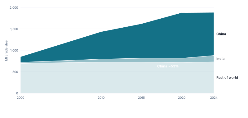
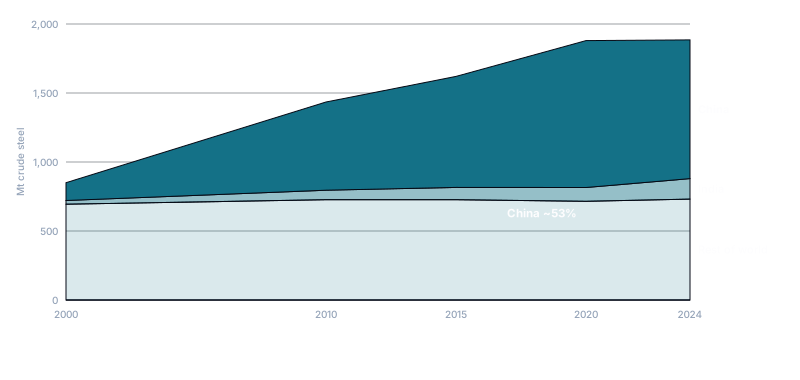
Figure data: Table 9.

2.3 Supply: producing countries

The supply map separates production from exportable supply. India, China, Iran and Russia mine large tonnages that mostly stay at home; the seaborne market that sets the price is dominated by Australia and Brazil, which mined 54% of the world’s ore in 2025 and shipped 74% of its exports in 2024 (Section 2.6). Over the decade the growth came from Australia (+20% since 2015), India (+99%) and Iran (+244%), while China’s own output fell 23% as its mines, at the bottom of the grade ladder, lost ground to imports. World output rose 14% from 2015 to 2025, to 2,600 Mt; it has held at about 2.5–2.6 Gt a year since 2022, below the 2,680 Mt of 2021.

Table 10. Iron ore mine production by country, 2015–2025 (Mt usable ore)

Source: USGS, Mineral Commodity Summaries, Iron Ore chapter, World Mine Production and Reserves, “Usable ore” — each year from the edition two years later, its revised column (2017, 2018, 2019, 2020, 2021, 2022, 2023, 2024, 2025 and 2026 editions); 2025 is the 2026 edition’s estimate. The 2017 and 2018 editions print million tons, later editions thousand tons, shown here in Mt; Rest of world = world total less the rows shown, computed here. The usable-ore basis starts with the 2017 edition, which is why the series starts in 2015 (Section 1.2). The Trend column is this guide’s judgement.

Figure 8. Leading iron ore mining countries, 2025 (Mt usable ore)

Figure data: Table 10, 2025 column.

Figure 9. World iron ore mine production, 2015–2025 (Mt usable ore)

Figure data: Table 10, World row.

Reserves make iron ore the least scarce commodity in this series. The USGS counts 200 Gt of crude ore holding 87 Gt of iron, and resources above 900 Gt. Australia holds 59 Gt of crude ore (24 Gt of it reported to the Australian JORC code), Russia 35 Gt and Brazil 34 Gt. Scarcity lives elsewhere: in grade (high-grade, low-impurity ore depletes much faster than the headline number, and the Pilbara’s shipped grade has drifted down), in infrastructure (a new district needs a railway and a port before its first tonne) and in DR-grade ore, of which the world has too little for its low-carbon steel plans. On an iron-content basis China’s reserves last 17 years and India’s 18 at 2025 output, against 45 for Australia and 58 for Brazil.

Table 11. Iron ore reserves by country, and reserve life

Notes to Table 11

1. Derived · reserves of iron content ÷ 2025e mine production of iron content, both from the same table. Very long lives (Russia, Mauritania) mean reserves far larger than current mining, not a measure of future supply.
2. Of Australia’s figure, 24 Gt of crude ore and 10 Gt of iron are reported to the JORC code or an equivalent.
3. Ukraine’s reserves are the A and B categories of the Soviet classification.

Source: USGS Mineral Commodity Summaries 2026: Iron Ore, World Mine Production and Reserves, “Reserves” (million metric tons, crude ore and iron content) and “Iron content” production 2025e, with footnotes 6 and 7, p.109; World Resources, p.109. Shares and reserve lives are computed here. Reserves are estimates and are revised between editions.

2.4 The supply–demand balance

No study group publishes an iron ore balance, so the market is read through China’s imports, the demand spine, and Chinese port inventories, the visible buffer, against the cost of the marginal tonne. When seaborne supply outruns what Chinese mills take, ore piles up at the ports and the price falls toward the cost of the highest-cost producers still running — Chinese domestic mines and small seaborne suppliers; when mills restock or supply stumbles (a dam failure, a cyclone at Port Hedland), stocks draw and the price jumps. No primary source publishes the marginal cost itself; the Australian Government expects falling prices “might result in the exit of high-cost producers”, and the published unit costs of the large producers are compared in Section 4.2.

China’s imports rose 30% from 2015 to 2024, to a record 1,238 Mt, even as its steel output peaked, because imported ore kept displacing its own low-grade mines. On worldsteel’s provisional 2025 trade matrix they reached about 1,315 Mt; the Australian Government counts 1,260 Mt on a dry basis. Port stocks tracked the surplus: Mysteel’s survey of 45 ports put them at 159.7 Mt at the end of 2025 — above the 158.6 Mt of a week earlier, which Mysteel called the highest since March 2022 — about six weeks of imports, and its enlarged 47-port survey showed 173.2 Mt in early October 2026. The price eased in step, from $162 in 2021 to $100 in 2025 (Table 3). What has not happened is a collapse: Chinese mills’ preference for imported grades, the majors’ cost positions and their restraint on volume have so far absorbed each increment of supply. Simandou is the stress test ahead.

Table 12. China’s iron ore imports and the visible buffer, 2015–2025

Notes to Table 12

1. Actual weight. 2015–2024 from each year’s “Iron ore” table in World Steel in Figures (the edition two years later); 2025 from worldsteel’s 2025 trade matrix, a provisional figure on a different compilation; the Australian Government prints 1,260 Mt for 2025 on a dry basis and calls China 75% of seaborne supply; China took 73.3% of world imports in 2024 (Table 17).
2. Port stocks (Mysteel weekly survey): 155.1 Mt by 18 December 2025 and 159.7 Mt by 31 December 2025 (45 ports); 173.2 Mt by 8 October 2026 (47 ports — the sample changed, so the two are not strictly comparable). Cover = 159.7 Mt ÷ (1,314.7 Mt ÷ 52) = 6.3 weeks of 2025 imports (6.6 weeks on the dry 1,260 Mt), computed here. n/o = not obtained (Section 8.1).

Source: worldsteel, World Steel in Figures, “Iron ore, {year}”, “Imports” column, row “China”, p.20 — editions 2017, 2018, 2019, 2020, 2021, 2022, 2023, 2024, 2025 and 2026 (2025 from “World trade in iron ore by area, 2025”, row “China”, “Total imports”, p.21); the trade tables are compiled for worldsteel by RMG Consulting. Port stocks from Mysteel’s weekly notes “China’s iron ore port stocks continue rising” (“stood at 159.7 million tonnes by December 31”), “China’s iron ore stocks at 45 ports top 155 mln t”, “China’s iron ore stocks at 45 ports climb further” (“also marked the highest level since March 2022”, of 158.6 Mt by 25 December) and “China’s iron ore port stocks rise further over holiday” (the free lead paragraphs). Australian figures: Resources and Energy Quarterly, September 2026, Table 3.2, p.38, and p.35. Share and cover are computed here.

Figure 10. China’s iron ore imports, 2015–2025 (Mt)

Figure data: Table 12; the 2025 column is worldsteel’s provisional matrix figure (note 1).

At the country level the market is one asymmetry with satellites. Australia exported 95% of its 2024 output and Brazil 87%; China imported 1,238 Mt to feed furnaces its own mines cannot supply; Japan, South Korea and Germany import almost all their ore; and India mines nearly all it uses, exporting a little.

Table 13. Iron ore production, trade and apparent consumption, major countries, 2024 (Mt)

Notes to Table 13

1. worldsteel adjusts China’s production “so that Fe content is similar to world average”; the USGS counts 293 Mt of usable ore for 2024.

Source: worldsteel World Steel in Figures 2026, “Iron ore, 2024” (million tonnes, actual weight; compiled by RMG Consulting), columns “Production”, “Exports”, “Imports” and “Apparent consumption”, p.20. Net exports = exports − imports, computed here. World exports and imports differ because of timing and reporting gaps.

Figure 11. Iron ore net trade, 2024 (Mt)

Figure data: Table 13, net exports column.

2.5 Supply structure: primary ore, grades & scrap

Iron is mined for its own sake: there is no meaningful by-product iron ore supply, so the supply-structure question is about grades and about the one large secondary source, scrap. Steelmakers draw their iron from three places — pig iron from ore, DRI from ore, and recycled steel — and scrap is the ore market’s long-run competitor: every tonne of the world’s growing steel stock is a future EAF charge. The Bureau of International Recycling estimates that some 630 Mt of recycled steel is used each year; in its seven key countries and regions, which make about 76% of world steel, scrap use was 461 Mt in 2024. China melted 210 Mt, only 20.9% of its crude steel, against 59% in the EU, 69% in the United States and 85% in Türkiye — the gap that a maturing Chinese scrap pool will close over time. The USGS puts the saving at 1.1 tonnes of iron ore for every tonne of steel recycled.

Table 14. Where steelmakers’ iron comes from

Notes to Table 14

1. BIR’s annual approximation, not a measured 2025 figure, so the shares are indicative; scrap and pig iron are not one-for-one in iron content.

Source: worldsteel World Steel in Figures 2026, Pig iron, p.18, and Direct reduced iron production, p.19, “World” 2025; Bureau of International Recycling, World Steel Recycling in Figures 2020–2024 (16th edition), “some 630 million tonnes of recycled steel are used each year in global steel production”, p.4, the seven-region total, p.2, and the country shares, p.5; USGS Mineral Commodity Summaries 2026: Iron and Steel Scrap, Recycling, “Recycling 1 ton of steel conserves 1.1 tons of iron ore”, p.104. Shares are computed here; the Trend and Response columns are this guide’s judgement.

Within primary ore, supply is graded like an examination. At the top sit DR-grade concentrates and pellets at about 67% Fe — Minas-Rio, Iron Bridge, LKAB, the Labrador Trough — scarce and increasingly bid for by low-carbon steel projects. Next come the high-grade fines of Carajás and Simandou at about 65%. The broad middle is the Pilbara blends at 60–62% — the benchmark itself. Below them sit discounted grades such as Fortescue’s 57%, which do well when steel margins are thin (mills chase cheap iron units) and badly when margins are fat (mills chase productivity). At the bottom are China’s low-grade mines, which must be upgraded into concentrate at high cost.

Table 15. The iron ore quality ladder

Source: the producers’ reserve and product statements, as in Tables 5 and 20 — Anglo American IAR 2025, Estimated Ore Reserves, p.370; Fortescue AR FY2025, Ore Reserves — Magnetite, p.47, and — Hematite, p.46; Vale 20-F 2025, Iron Ore Mineral Reserves, p.90; Rio Tinto AR 2025, Ore Reserves, pp.288–289, and Iron Ore, p.31; BHP AR FY2025, Ore Reserves, p.213; Champion AR FY2025, Table 7, p.121; Cliffs 10-K FY2025, Iron Ore Mineral Reserves, p.37; LKAB ASR 2025, Iron Mineral Reserves, pdf p.202. Grades are as filed (product or in-situ reserve); the segments and economics are this guide’s summary.

2.6 Trade flows & the iron highway

Iron ore is the ocean’s largest dry-bulk cargo, and its map is simple: two loading coasts, one destination. From the Pilbara’s ports — Port Hedland, Dampier and Cape Lambert — capesize ships run north to China on the C5 route; from Brazil’s Ponta da Madeira and Tubarão the C3 route runs around the Cape of Good Hope, a much longer haul offset by Carajás grade and Vale’s fleet of 400,000-tonne Valemax carriers. Freight from Western Australia to northern China averaged about $18 a tonne in the September quarter of 2026, by the Australian Government’s count. Around the main line sit South Africa’s Saldanha Bay, Canada’s Sept-Îles, Sweden’s Narvik and Luleå — serving Europe — and now Simandou’s ports in Guinea.

Table 16. Largest iron ore exporters, 2024

Notes to Table 16

1. A regional row in worldsteel’s table, so no single Comtrade value applies (n/c); Ukraine alone reported $2.8 bn of exports.
2. China’s exports are small against its 1,238 Mt of imports (Table 17).
3. Values as exporters declared them to UN Comtrade, FOB.

Source: volumes from worldsteel World Steel in Figures 2026, “Iron ore, 2024”, “Exports” column, p.20 (actual weight); values from UN Comtrade, HS 2601 (iron ores and concentrates), annual 2024, flow X, partner World, every reporter — exports query, field “primaryValue”. Shares are computed here from worldsteel’s world total.

Table 17. Largest iron ore importers, 2024

Notes to Table 17

1. The Netherlands is a transit hub (Rotterdam); it also exported 18.6 Mt.
2. Values as importers declared them to UN Comtrade, CIF (including freight and insurance), so world imports exceed world exports in value (Table 16).

Source: volumes from worldsteel World Steel in Figures 2026, “Iron ore, 2024”, “Imports” column, p.20 (actual weight); values from UN Comtrade, HS 2601, annual 2024, flow M, partner World, every reporter — imports query, field “primaryValue”. Shares are computed here from worldsteel’s world total.

The 2025 trade matrix shows where the ore went and how concentrated the routes are: Oceania sent 794 Mt to China, 60% of China’s imports, and South America 312 Mt, 24%.

Table 18. World iron ore trade by region, 2025 — the main flows (Mt)

Source: worldsteel World Steel in Figures 2026, “World trade in iron ore by area, 2025” (million tonnes), p.21 — rows are importing regions and columns exporting regions in the original, transposed here; flows under 10 Mt are not shown (n/s) but are included in the totals; the world total includes destinations not shown (Other Europe, North and South America, the CIS, Oceania).

Figure 12. Where iron ore travels: exporting and importing regions, 2025 (Mt)

Figure data: Table 18 — every flow of 25 Mt or more; bars show each region’s total on one scale; the highlighted route is Oceania to China.

There is no Hormuz here: iron ore’s chokepoints are port-rail systems — a cyclone at Port Hedland or a stoppage on a Carajás railway moves the world price — and the demand-side concentration itself, with three-quarters of seaborne ore sailing to one country. Weather, dam safety and Chinese policy are the trade’s disruption risks, not straits.

2.7 Market organisations & supply coordination

Iron ore’s coordination story is a pendulum between producer and consumer power. For forty years the annual benchmark was the coordination — a negotiation between a few miners and a few steelmakers — until it ended in 2010. The index era left a structural oligopoly: four producers whose capital discipline since the 2012–15 bust works as informal supply management. Together they produced about 1.15 Gt in 2025 or fiscal 2025 — roughly two-thirds of world exports, though their bases differ (Table 19). The consumer side has organised in response. China Mineral Resources Group (CMRG), a centralised buyer for Chinese mills, now negotiates purchases and supply agreements with the miners; the Australian Government notes its “growing presence in the seaborne iron ore market” and possible “implications for commercial negotiations and price discovery”. Beijing’s wider toolkit — steel-output controls and state backing for Simandou, where Chinese groups hold 47% of SimFer’s holding company and 49% of the WCS mine and infrastructure — points the same way: loosening the Australian–Brazilian grip on the marginal tonne. Around this contest the formal institutions are light: worldsteel publishes statistics, and there is no study group and no government stockpile of consequence (the USGS lists none for the United States).

Table 19. Concentration and coordination in iron ore

Notes to Table 19

1. Vale 336.1 Mt (2025, including 31.2 Mt bought from third parties), Rio Tinto Pilbara 327.3 Mt (2025, 100%), BHP WAIO 290 Mt (year to June 2025, 100%) and Fortescue 198.4 Mt shipped (year to June 2025); the sum mixes years and bases and includes ore sold domestically, so the share of exports is approximate.

Source: shares from worldsteel World Steel in Figures 2026, “Iron ore, 2024”, p.20 (computed here); company output from Table 20; CMRG and Simandou from the Australian Government’s Resources and Energy Quarterly, September 2026, pp.34–35 (“growing presence in the seaborne iron ore market”; Simandou “reaching up to 120 Mt a year by 2030”) and the Rio Tinto Annual Report 2025, Simandou ownership, p.23. The Role and Leverage columns are this guide’s judgement.

3. The companies & the value chain

3.1 The largest iron ore companies

Four companies define the industry. Vale produced 336 Mt in 2025, including 31 Mt bought from third parties; Rio Tinto’s Pilbara network produced 327 Mt at 100%; BHP’s WAIO a record 290 Mt at 100% in its year to June 2025; and Fortescue — the only pure play among them — shipped 198 Mt. Their economics are the envy of mining: integrated mine-rail-port systems and unit costs of $18–24 a tonne (Section 4.2). Behind them come Anglo American (Kumba in South Africa and Minas-Rio in Brazil, 61 Mt), state-owned LKAB in Sweden, which produced 86% of the iron ore mined in the EU in 2025, North America’s pellet and concentrate producers (Cleveland-Cliffs, Champion Iron), private Hancock Prospecting’s Roy Hill, which publishes no figures, and India’s NMDC. Reserve lives differ widely: about 8 years for Rio Tinto’s Pilbara at 2025 output, 14 for WAIO and 32 for Vale’s Northern System. Note what the line-up means for investors: apart from Fortescue and a few mid-caps, iron ore comes bundled inside diversified majors, so the purity of the exposure is itself a screening variable. Companies here are compared on production, reserves and cost, never market capitalisation — screen them all on Metal Pilot’s iron ore mining stock screener.

Table 20. Largest iron ore producers by output and reserves

Notes to Table 20

1. Each company’s own basis: Vale total production including third-party purchases; Rio Tinto Pilbara and BHP WAIO at 100%; Fortescue shipments in wet tonnes; Anglo American 100% of Kumba and Minas-Rio; Cliffs its share, converted from 17 million long tons. Calendar 2025, except BHP and Fortescue (years to 30 June 2025) and Champion (year to 31 March 2025).
2. Proved plus Probable, 100% basis. Vale’s are in-situ ore including moisture; Rio Tinto’s, BHP’s, Fortescue’s and Anglo American’s are marketable or saleable product; LKAB’s, Cliffs’s and Champion’s are crude ore. LKAB’s total is not printed in the rows read.
3. Derived · 2,082 Mlt × the filed 32% process recovery ÷ 17 Mlt; 2025 output was depressed by idled mines. Reserve life is computed only where reserves and production share a basis (n/c otherwise); Rio Tinto 2,616 ÷ 327.3, BHP 4,050 ÷ 290 and Vale 5,479.4 ÷ 170.2, computed here; Kumba’s and Minas-Rio’s are the filed figures.

Source: the companies’ 2025 reports, row by row as cited — Vale Form 20-F 2025, Rio Tinto Annual Report 2025, BHP Annual Report 2025, Fortescue FY25 Annual Report, Anglo American Integrated Annual Report 2025, LKAB Annual and Sustainability Report 2025, Cleveland-Cliffs Form 10-K 2025 and Champion Iron Annual Report FY2025. Listing notes: LKAB is wholly owned by the Swedish state; Kumba is majority-owned by Anglo American; Hancock Prospecting is private; the WCS side of Simandou sits in unlisted consortium companies. NMDC (India) is omitted because its report could not be retrieved. No market-capitalisation figures are shown by design.

Figure 13. Iron ore output by company, 2025 or fiscal 2025 (Mt)

Figure data: Table 20; each bar is the company’s own basis (Table 20, note 1), so the bars rank scale, not like-for-like output.

3.2 Company archetypes along the value chain

Iron ore’s business models sort by cost position and by what else the company does. The low-cost majors in the Pilbara and Carajás are the archetype the industry is built on: bottom-of-the-curve costs, infrastructure moats and margins that have survived every annual price this century — inside diversified groups that dilute the exposure. The pure-play producer (Fortescue, Champion, Kumba as a listed company) offers undiluted price leverage, and undiluted pain in busts. High-cost swing producers — China’s domestic mines and small seaborne suppliers — set the marginal cost and live or die by the cycle. Pellet and DR-feed specialists (LKAB, Minas-Rio, Iron Bridge) sell grade and processing rather than bulk tonnes and stand to gain from low-carbon steel. Developers face iron ore’s brutal entry ticket: a new district needs a railway and a port before its first tonne — Simandou needed more than 600 km of new railway and two ports before its first shipment in December 2025. Integrated miner-steelmakers (Cleveland-Cliffs, much of China’s industry) internalise the ore price. Iron ore has no meaningful royalty or streaming layer: the producers fund their own systems.

Table 21. Iron ore company archetypes

Source: this guide’s classification of the companies in Table 20, from their reports — Rio Tinto AR 2025, BHP AR FY2025, Vale 20-F 2025, Fortescue AR FY2025, Anglo American IAR 2025, LKAB ASR 2025, Cliffs 10-K FY2025 and Champion AR FY2025 (unit costs in Table 25). All columns other than Examples are judgement.

3.3 Infrastructure & balance-sheet assets

An iron ore company’s balance sheet is mostly logistics with a mining licence. The ore body is described by tonnage, grade, impurities and strip ratio — but reserves are rarely the constraint. The value sits in the system: heavy-haul railways, port capacity (berth and channel allocations cap output in the Pilbara), rolling stock and processing plants — concentrators for magnetite, pellet plants and, increasingly, DRI and briquetting plants. Read capacity, utilisation and expansion cost for each link: the market prices a system’s tightest link, not its pit. Iron ore adds two balance-sheet items rarer elsewhere. Tailings liabilities: after Brumadinho, Vale has de-characterised 19 of the 30 upstream dams it had in 2019 and carried a $2.1 billion provision for the rest at the end of 2025, and the 2024 settlement over the Samarco dam failure is valued at R$170 billion on a 100% basis (Section 4.5). And quality trajectory: a system whose shipped grade is drifting down — as the Pilbara’s is — is quietly losing its premium.

Table 22. Iron ore company asset types and metrics

Source: this guide’s summary of the asset disclosures in the reports cited under Table 20 — for example the Rio Tinto AR 2025 and the Vale 20-F 2025, which also gives the tailings provision — and the reserve-reporting codes they follow (JORC in Australia, SEC S-K 1300 in the United States, NI 43-101 in Canada).

4. Investing in iron

4.1 Ways to own it — exposure vehicles

Physical iron ore is the least ownable commodity in this series — nobody stores capesize cargoes for investment — so exposure is financial or corporate. Futures exist and are liquid: SGX’s cash-settled contracts are the international professional venue and DCE’s physically delivered contract dominates inside China. Both are institutional tools; no major retail fund tracks iron ore futures, so the roll-yield trap that hurts commodity-fund buyers elsewhere — a futures fund must sell expiring contracts and buy later ones, which costs money when later contracts are dearer (contango) and earns it when they are cheaper (backwardation) — is a professional’s concern here; the oil guide shows how it played out in the 2020 crash. For everyone else the route is equities, along a purity spectrum: Fortescue and the mid-cap pure plays offer direct leverage; Vale is iron-ore-led but carries base metals and Brazilian risk; Rio Tinto and BHP wrap world-class iron ore inside diversified portfolios; Cleveland-Cliffs ties ore to US steel. Broad mining funds are the collective proxy. One structural note: because the majors have paid out much of iron ore’s cash flow since the 2015 bust rather than chasing volume, their shares behave as dividend payers with cyclical capital — the income flexes with the price.

Table 23. Ways to own iron ore

Source: the exchanges’ product pages — SGX iron ore and DCE (Products → Iron Ore) — for the settlement type; the companies’ reports (Table 20) for the business mix. Structural attributes only — no fees or prices, which change; the columns are this guide’s judgement.

4.2 How to value & screen iron ore producers

Iron ore screening is margin arithmetic plus quality foresight. Start where the cash is made: unit cost against the price. The four majors publish costs of $18.0–23.5 a tonne for 2025 or fiscal 2025, against an Australian export price that averaged $87 in 2025 — margins most miners never see. Compare producers on realised price, not the benchmark: a 57% Fe seller earns well below the index and a 65% seller above it, and freight separates Brazil from Australia. Then quality trajectory: the grade and impurity path of the reserves decides whether a producer’s discount widens or narrows over a decade — the most underrated variable in the sector. Then system headroom: growth within existing rail and port capacity is cheap, while a new district is a different business. Round out the screen with dividend policy and capital discipline, tailings and jurisdiction liabilities, and low-carbon positioning — DR-grade resources, pellet capacity and partnerships with DRI projects are the growth options in an ex-growth market. These are the screens — production, reserves, grade and cost — you can run across every listed producer on Metal Pilot’s iron ore mining stock screener.

Table 24. Iron ore producer screening metrics

Source: this guide’s screening framework, built on the disclosures in Table 20 — unit costs, reserves and grades from the Rio Tinto AR 2025, BHP AR FY2025, Vale 20-F 2025 and Fortescue AR FY2025; the ranges are judgement.

Table 25. Unit costs of iron ore producers that publish one, 2025 or fiscal 2025

Notes to Table 25

1. The bases are not comparable. Mine-gate C1 costs (Fortescue, BHP, Vale, Rio Tinto, Champion) exclude freight, royalties and sustaining capital; Anglo American’s FOB costs include rail and port; Fortescue’s are per wet tonne. Vale’s all-in cost, which adds freight, royalties and overheads, was $54.2/t (Vale AR 2025, p.4). Champion’s 65%-plus concentrate earns a premium that its cost partly reflects. Years as in Table 20.

Source: the producers’ 2025 reports, row by row as cited — Fortescue FY25 Annual Report, BHP Annual Report 2025, Vale Annual Report 2025 (Investors → Results and reports → Annual Report 2025), Rio Tinto Annual Report 2025, Anglo American Integrated Annual Report 2025 and Champion Iron Annual Report FY2025. Output is each producer’s basis from Tables 5 and 20 (Vale’s own production, excluding purchases).

Figure 14. Cost curve of seven iron ore producers, 2025 or fiscal 2025 (US$/t)

Figure data: Table 25, seven producers ranked by unit cost, bar widths their share of the seven’s 1,188 Mt; the dashed line is the 2025 average Australian export price, $87 a tonne FOB (Resources and Energy Quarterly, September 2026, Table 3.3, p.39). The bases differ (Table 25, note 1), so the curve ranks the published figures rather than a common cost.

4.3 Macro regimes, rates & correlations

Iron ore is the China cycle distilled — more so than copper, because it lacks copper’s electrification demand and half its market is one country’s steel industry. (For how the whole commodity complex behaves across the same regimes, see the macro regime guide.) The regime map is lopsided. Iron ore does best in Chinese stimulus and construction booms: the annual average rose 82% in 2010, after Beijing’s 2009 stimulus, and 48% in 2021. It does well in global expansions (from $25 in 2004 to $123 in 2007) and supply shocks (up 58% from January to July 2019 after Brumadinho). It does worst in its own supply waves — down 67% from 2011 to 2015 as boom-era mines arrived — in Chinese property and credit retrenchment (down 38% from 2021 to 2025 through China’s property slump) and in global recessions (down 49% in 2009, when the S&P 500’s annual average fell 22.3%). Interest rates and the dollar act through the usual channels — a dollar-priced commodity weakens when the dollar strengthens, as in 2015, when the broad dollar index rose 13% and ore fell 42% — but they are second-order next to Chinese steel output. What distinguishes iron ore is the margin cushion: because the majors’ costs sit so far below any recent price, bear markets crush the price long before they threaten the core producers, and the cycle moves wealth between miners and mills rather than switching mines off, except at the high-cost fringe.

Table 26. Iron ore across economic regimes

Source: Table 3 and the World Bank monthly series; the S&P 500 from CNBC chart data and the broad dollar from FRED DTWEXBGS, as annual averages of daily values. Changes are computed here; the regime labels and the Why column are this guide’s judgement and are historical, not predictive.

On past performance, iron ore delivered the greatest commodity trade of the century’s first decade — a near nine-fold rise in the annual average from 2000 to 2011 — and then the standard lesson: the 2011–2015 bust took the annual average from $167.8 to $55.9 (−67%) and the monthly average from $187.2 in February 2011 to $40.5 in December 2015 (−78%). The equity amplifier is that concluded episode. Vale’s New York-listed shares fell 94% from their January 2011 peak close to their January 2016 trough; Cleveland-Cliffs, then a leveraged high-cost producer, fell 99%; Fortescue fell 80%, BHP 81% and Rio Tinto 70%. On annual averages, 2011 to 2015, the ranking matched the cost curve: Cliffs −95%, Vale −81%, Fortescue −64%, BHP −53%, Rio Tinto −36%. The recovery paid the survivors: from the 2016 trough to their 2021 highs Fortescue rose about 18-fold and Vale about 11-fold. Over the whole of 2000–2025 the iron ore price rose 434% in nominal terms against 87% for US consumer prices — about 2.9 times in real terms, though the start is the converted contract price and the end a spot price (Table 3, note 1). Past performance is not indicative of future results.

On correlations (monthly log changes, January 2010 to December 2025 — the index era, 192 months): iron ore moves with copper (+0.45, the shared China engine) and with the Australian dollar (+0.35 — ore is Australia’s largest export), against the US dollar (−0.30), and only weakly with US equities (+0.16), gold (+0.16) and US inflation (+0.08). The links have drifted: from 2010–2017 to 2018–2025 the Australian dollar’s correlation rose from +0.31 to +0.40 and the US dollar’s from −0.23 to −0.37, while copper’s held at about +0.45. Its tightest links are Chinese — steel margins, property starts and port stocks — for which no free monthly series is used here. All correlations weaken in supply shocks, which are iron-ore-specific by nature.

Table 27. Iron ore correlations, monthly, 2010–2025

Source: computed here — Pearson correlations of monthly log changes in monthly averages — from the World Bank monthly series (“Iron ore, cfr spot”, “Copper”, “Gold”), FRED DEXUSAL, DTWEXBGS and CPIAUCSL, and CNBC chart data for the S&P 500. Correlations are sample-dependent and time-varying, and break down in supply shocks; the Note column is this guide’s judgement.

Figure 15. Iron ore’s correlations with major assets, monthly, 2010–2025

Figure data: Table 27, five of its six assets (US CPI, +0.08, is in the table only). Tiles are shaded on a fixed scale with 0.75 as full strength.

4.4 Price drivers & cycles

The durable drivers, read through concluded episodes. On the demand side: Chinese steel output — hot-metal production explains most of the price’s swings — steel-mill margins (profitable mills chase high-grade ore; loss-making mills chase discounts) and the long shadow of scrap. On the supply side: the investment cycle of the majors (the expansions of 2011–14 built the tonnes that crushed 2015), disruption risk concentrated in two countries’ logistics (cyclones, dam failures) and the marginal cost of China’s own mines. The settled case studies: the 2000–2011 supercycle — Chinese steel output nearly quadrupled by 2008 and the price rose about nine-fold, destroying the benchmark system on the way — proof of how far a bulk commodity can travel when the world’s most populous country industrialises. The 2011–2015 bust — the majors’ boom-era expansions landing in a slowing China; the price down two-thirds, Vale’s shares down 94% — proof that in iron ore the cost curve is destiny. Brumadinho (January 2019) — a tailings dam failure that killed 270 people and lifted the price 58% in six months — proof of supply concentration, and the industry’s moral low point. And the 2020–21 stimulus round trip — a June 2021 average of $214, then $96 by November, a 55% fall, after Beijing ordered steel output curbed — proof that the demand side has an administrator. Simandou’s ramp and CMRG’s buying are the live continuation, noted as current context rather than settled history.

Figure 16. Seven episodes that shaped the iron ore market, 2008–2021

Chart source: price moves from Table 3 and the World Bank monthly series; steel output from Table 9; the 2010 benchmark change from USGS Mineral Industry Surveys: Iron Ore in May 2010, p.1; the dam failures from the Vale Form 20-F 2025, pp.11 and 13. The selection of episodes is this guide’s.

Table 28. Iron ore price drivers

Source: this guide’s synthesis of Sections 2 and 4 — prices from the World Bank Pink Sheet (Table 3), steel and trade from worldsteel World Steel in Figures 2026 (Tables 9, 12) and unit costs from the producers’ reports (Table 25). The drivers are judgement; the evidence is the concluded episodes above.

4.5 Risks, controversies & ESG

Iron ore’s risk register starts with its greatest strength turned around: concentration. Demand concentration means one Chinese policy decision — a steel-output cap, a property credit squeeze, a change in state purchasing — can reprice the market; supply concentration means the reverse (a dam, a cyclone). The structural bear case is demographic: much of China’s built environment is built, its scrap pool is filling, and the Australian Government projects Chinese imports falling to 1,152 Mt by 2031; the argument is about the slope, not the direction. Simandou cuts both ways: for the market it is up to 120 Mt of new high-grade supply into a plateauing demand base; for its owners it is Guinean political risk on a single rail corridor of more than 600 km.

The ESG ledger is dominated by one word: tailings. The failures of Samarco’s Fundão dam (November 2015, 19 deaths) and Vale’s Brumadinho dam (January 2019, 270 deaths) — both upstream-type dams — are among the deadliest mining disasters of the century. The 2024 settlement over Fundão is valued at R$170 billion (about US$32 billion) on a 100% basis, Vale has de-characterised 19 of its 30 upstream dams, and the industry adopted an international tailings standard. The second word is carbon: steelmaking accounts for 7–8% of global greenhouse-gas emissions by worldsteel’s estimate — about 2.18 tonnes of CO₂-equivalent per tonne of steel in 2024 — and those emissions are the mills’ (the miners’ Scope 3), which is why low-carbon steel partnerships and DR-grade projects now shape miners’ strategies. The counterweights: mining iron ore is low-intensity per tonne, dam practices improved after 2019, and steel is endlessly recyclable — the long-run answer to its own emissions. These are contested questions, and reasonable analysts weigh them differently.

Figure 17. Iron ore risk map — likelihood vs. impact

Chart source: this guide’s qualitative assessment of the risks discussed in Section 4.5; positions are judgement, not data.

5. Future outlook & forecasts

Iron ore’s outlook question is unusual in this series: not whether demand grows — the agencies expect it not to — but how the world’s most profitable mining business manages an ex-growth market. Forecasts are scenarios, not measured facts, and they hinge on two hard-to-predict institutions: the Chinese state and the capital discipline of four boards.

5.1 Demand

worldsteel expects world steel demand to grow just 0.3% in 2026 and 2.2% in 2027, to 1,762 Mt — and warns of material downward revisions if the Middle East conflict persists — with China down 1.5% in 2026 and flat in 2027 and India up 7–9% a year. The Australian Government sees Chinese crude steel output falling from 961 Mt in 2025 to 933 Mt in 2026–27 and 926 Mt in 2031, and China’s ore imports declining from 1,260 Mt to 1,152 Mt by 2031. Beneath the totals, the EAF share keeps rising (above 34% by 2031) and India grows, though much of its steel will be fed by Indian ore. The qualitative shift is more investable than the quantitative one: demand for DR-grade ore and pellets — the feed for gas- and hydrogen-based DRI plants in Europe, the Gulf and eventually China — is set to grow from a small base, splitting the market into a shrinking bulk segment and a growing quality segment.

5.2 Supply and the balance

Supply is doing what it does at cycle turns: arriving. Rio Tinto expects a 30-month ramp to full capacity at Simandou after rail-to-port commissioning around the end of the first quarter of 2026, with its own port commissioning in early 2027; the Australian Government expects exports of up to 120 Mt a year by 2030 at 65–68% Fe, and its “Other Africa” exports — mostly Guinea — rising from 34 Mt in 2025 to 159 Mt in 2031. World trade grows only modestly (1,744 Mt in 2025 to 1,838 Mt in 2031), so the new tonnes displace others: Australian exports ease to 905 Mt by 2031 and the forecast FOB price falls from $87 in 2025 to $70 in 2031 in nominal terms. The wildcards: Chinese stimulus (any serious property support would rerun 2020–21 in miniature), the majors’ volume discipline, disruption (the sector’s permanent upside risk) and faster low-carbon steel policy, which would tighten the premium segment whatever the bulk balance.

Table 29. Iron ore outlook indicators (scenario figures)

Notes to Table 29

1. worldsteel’s apparent steel use for 2025 (finished steel), from World Steel in Figures 2026, p.16; the outlook’s growth rates apply to its own 2025 estimate.
2. 62% Fe for 2025; 61% Fe from 2026, after the change of benchmark basis.

Source: worldsteel, “worldsteel Short Range Outlook April 2026” (press release; the October 2026 outlook was not yet published at the data date); the Australian Government’s Resources and Energy Quarterly, September 2026, Table 3.1 (p.37), Table 3.2 (p.38), Table 3.3 (p.39) and pp.33–34; Rio Tinto Annual Report 2025, Simandou, pp.21 and 31. “z” years in REQ are projections; all figures are scenarios, not measured data.

5.3 Catalysts to watch

The watch-list is short and Chinese-weighted. Near term: Chinese hot-metal output and steel margins (the demand pulse), property-stimulus decisions, port inventories (the visible balance), the Simandou ramp (each commissioning milestone is supply news), CMRG’s negotiating behaviour and the Pilbara cyclone season. Structurally: the majors’ volume discipline as the surplus builds, India’s steel and ore path, the EAF and scrap share in Chinese policy, and the pace of DRI investment in Europe and the Gulf, which sets the slope of the DR-grade premium. What would confirm the bear case: Simandou ramping on schedule into flat Chinese demand with no supply response elsewhere. What would break it: a genuine Chinese property recovery, a major supply disruption, or coordinated volume restraint.

Table 30. Iron ore catalyst calendar

Source: Rio Tinto Annual Report 2025, Simandou, p.21; the Australian Government’s Resources and Energy Quarterly, September 2026, p.34 and Table 3.2, p.38; the publishers’ release patterns (worldsteel, USGS, Mysteel). The Why and Watch columns are this guide’s judgement.

Figure 18. Iron ore catalysts, near term to 2031

Figure data: Table 30, the dated catalysts; the ramp-up end (2028) is Rio Tinto’s 30-month ramp counted from the end of the first quarter of 2026.

6. Summary

Iron ore is the raw material of steel — about 2.6 Gt mined in 2025, most of it becoming the 1,849 Mt of crude steel that frames every economy. It comes from banded iron formations concentrated in a few districts — Australia (38% of world output, mostly from the Pilbara) and Brazil’s Carajás and Iron Quadrangle, now joined by Guinea’s Simandou — and is priced on a daily CFR China index that replaced annual negotiated benchmarks in 2010 and moved from a 62% to a 61% Fe basis in 2026. That price traces the century’s defining commodity arc: about $19 a tonne in 2000, $168 in 2011, $56 in 2015, $162 in 2021 and $100 in 2025. The market is an oligopoly facing a monopsony: Australia and Brazil ship 74% of world exports and four companies dominate them, while China takes 75% of seaborne ore — 1,238 Mt in 2024 — increasingly through a centralised buyer, CMRG, with port stocks near 160 Mt, about six weeks of imports, as the visible balance. Demand is steel, and steel has plateaued: China’s output peaked in 2020, India grows, and the scrap-fed EAF route (30% of steel, above 34% by 2031) slowly erodes ore demand while creating a premium market for DR-grade ore. The companies are the cost curve in person — unit costs of $18–24 a tonne at the majors, screened on cost, grade trajectory and system headroom, never market capitalisation — and their shares amplify the cycle (Vale −94% and Cliffs −99% in the concluded 2011–2016 bust, in cost-curve order). The regime profile is the China cycle distilled: stimulus and supply shocks lift it; property retrenchment and supply waves sink it. The single variable to watch is Chinese steel against the Simandou-led supply wave, with the DR-grade premium as the structural story beneath the cycle.

To go from this big-picture view to the actual companies — screening every iron ore producer by production, reserves, grade and cost — explore Metal Pilot’s iron ore mining stock screener.

7. Vocabulary

Every specialised term used in this report, defined at first use in the body, collected here for reference.

Table 31. Iron ore vocabulary

Source: definitions follow the USGS Mineral Commodity Summaries 2026: Iron Ore, worldsteel World Steel in Figures 2026, the World Bank Pink Sheet’s iron ore definition and the producers’ reports in Table 20; the “why it matters” column is this guide’s judgement.

8. Sources, methodology & disclaimer

8.1 Sources, methodology & data vintage

Methodology. Data as of 10 October 2026; the guide is refreshed annually, after the USGS Mineral Commodity Summaries (February) and worldsteel’s World Steel in Figures (June), with the Australian Government’s quarterly outlook for the forecasts. Market structure is for full-year 2025; trade by country is for 2024, the latest year worldsteel prints by country, with its regional 2025 matrix for the routes; company figures are for calendar 2025 or the fiscal year ending in 2025 — 30 June for BHP and Fortescue, 31 March for Champion Iron; BHP’s and Fortescue’s years to June 2026, published in August 2026, enter at the next refresh. Prices are calendar-year and multi-year averages of the World Bank’s iron ore series, never spot quotes; 2000–2005 contract prices are converted from US cents per dmtu at 65.1% Fe (Table 3, note 1), and the trailing-twelve-month average is computed from the monthly series. Three counts are kept apart: the USGS for mine output by country, reserves and the 2015–2025 series (usable ore, each year from the edition two years later); worldsteel for steel, pig iron, DRI and ore trade (actual weight; its China production figure is Fe-adjusted); and the Australian Government for the outlook and the dry-basis 2025 China imports. Long tons are converted at 1.016 t. Correlations use monthly log changes of monthly averages, January 2010–December 2025; equity episodes use CNBC’s adjusted daily closes and their annual means, as percentage moves only. Every derived figure is computed in scripts kept with this guide’s evidence. Judgement columns are labelled. Reserves, resources and forecasts are estimates, not measured facts.

Data gaps & substitutions.

• Balance. No agency publishes an iron ore surplus or deficit series; China’s imports, port stocks and the cost curve stand in (Section 2.4), as the iron ore adaptation of this series prescribes.
• Consumption by country. Iron ore use is not surveyed; worldsteel’s apparent consumption (production + imports − exports) for 2024 is used (Table 13), with steel, pig iron and DRI by country for 2025 (Table 8).
• End use. No free agency source prints a global split of steel use by sector; the US split from the USGS is shown instead (Table 7).
• China’s imports. The 2015–2024 series is worldsteel’s (actual weight); 2025 is worldsteel’s provisional trade-matrix figure (1,314.7 Mt), against 1,260 Mt dry from the Australian Government. China’s customs series was not retrieved.
• Port stocks. Only Mysteel’s free weekly lead paragraphs are used; year-end levels before 2025 were not obtained, and the survey grew from 45 to 47 ports in 2026.
• Marginal cost. No primary source publishes the cost of China’s domestic mines; the published unit costs of seven producers are shown instead (Table 25), on bases that differ.
• Scrap. The global figure (about 630 Mt a year) is BIR’s approximation; the measured total covers seven regions.
• Companies. Bases differ (100% vs. attributable, wet vs. dry, calendar vs. fiscal years, product vs. crude-ore reserves). Hancock Prospecting publishes no figures; NMDC’s report could not be retrieved; Champion’s year to March 2026 was not read.
• Sources outside the hierarchy. Equity prices are CNBC’s adjusted daily closes, used for percentage moves only, because no free primary price history can be downloaded. The Platts subscriber note and the exchanges’ product pages refused scripted download and are cited live; the SGX and DCE contract specifications could not be read in full.
• Source conflicts. World mine output in 2024 is 2,600 Mt on the USGS count (usable ore) and 2,604.5 Mt in worldsteel’s table (actual weight, China Fe-adjusted); China’s 2024 output is 293 Mt (USGS) or 300.1 Mt (worldsteel). The guide uses each source for the tables named above and never mixes them in one row.

Refresh log.

• 10 Oct 2026 — full refresh. Moved every series to the newest editions (USGS MCS 2026 with each year’s latest revision, worldsteel World Steel in Figures 2026, the Australian Government’s September 2026 outlook, UN Comtrade 2024, the producers’ latest reports) and replaced the price series with the World Bank’s. Corrected the world production series, whose earlier figures mixed USGS bases (now 2,280 Mt for 2015 on the usable-ore basis, against about 2,110 Mt previously), and the 2025 average price ($100.2, against about $104 from the IMF series). Recorded IODEX’s move to a 61% Fe basis. Replaced approximate and aggregator-sourced figures — China’s imports, port stocks, net positions, company output and costs, correlations and equity moves — with agency, exchange and company data, and dropped figures no primary source supports (Chinese domestic costs, voyage days, CMRG’s purchasing pause). Added the steel-route, end-use, reserves, trade, unit-cost and outlook tables and the source register; rebuilt every chart as a component, including the steel chart that was an SVG.
• 6 Sep 2026 — first published (data as of 6 July 2026).

The register below is the guide’s reference list: one band per document, in order of first use, each linked to the edition cited.

Table 32. Source register — the document behind every table and figure

Source: compiled from the source lines under each table and figure in this guide; each band links the edition cited.

8.2 Disclaimer & disclosure

This report is for informational purposes only and is not investment advice, a recommendation, or an offer to buy or sell any security or commodity. Iron ore prices are volatile and policy-sensitive, and the figures here are estimates as of the stated date that will change; reserves, resources, correlations and regime observations are estimates and historical patterns that may not persist. Do your own research and consult a licensed financial adviser before acting. This report was prepared with the assistance of AI; its figures were sourced from the documents in the register and reviewed, but readers should verify any number before relying on it. The author holds no position disclosed as a conflict in respect of the companies named.